single area pi control in the frequency domain
My previous post saw the successful implementation of a single area power system simulation in MATLAB’s Simulink. This model used a proportional (P) feedback loop for controlling the system frequency when faced with a step change to load demand. As detailed in my post on primary controllers, this type of control is not able to restore the system frequency to the scheduled value - the simulation confirmed this analysis.
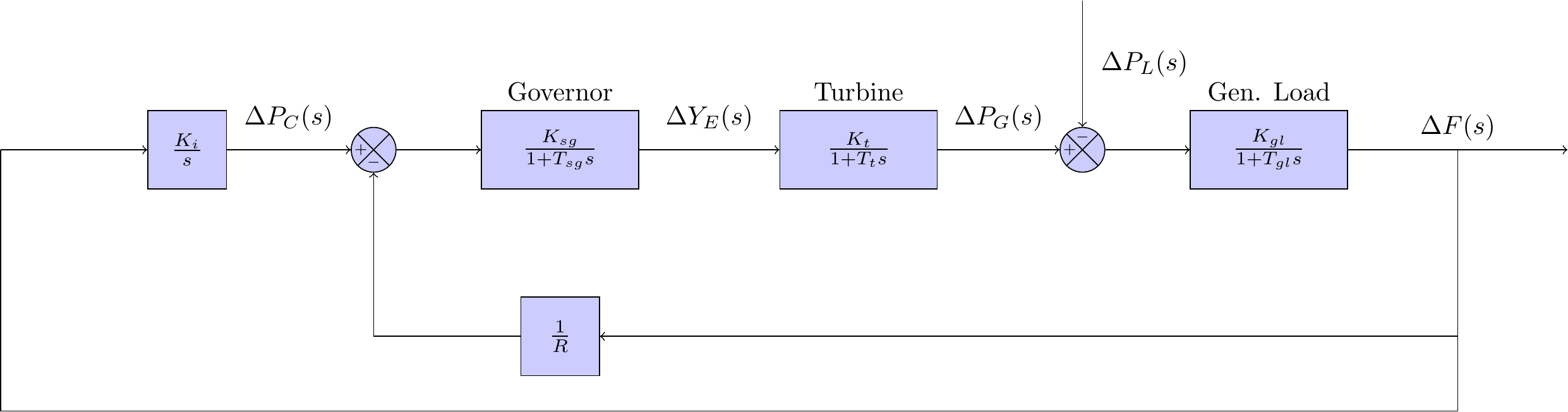
This post will be almost identical, except for the fact that an additional feedback loop will be added to the model. I have previously written about secondary control loops - this type of controller sees an integral feedback loop connected to the speed changer input . The block diagram can be seen in Figure 1 below.
MATLAB’s Simulink was used to implement this frequency domain model. The model parameter values are almost identical to the ones used in the previous post, which were selected from some of the more common values I have seen in the literature. A full breakdown of the model parameters, including a description and their assigned values, can be seen in Table 1.
| Description | Parameter | Value |
|---|---|---|
| Integral gain | \(K_{i}\) | -7.00 |
| Speed governor gain | \(K_{sg}\) | 1.00 |
| Speed governor time constant | \(T_{sg}\) | 0.20 |
| Turbine gain | \(K_{t}\) | 1.00 |
| Turbine time constant | \(T_{t}\) | 0.50 |
| Generator load gain | \(K_{gl}\) | 1.25 |
| Generator load time constant | \(T_{gl}\) | 12.5 |
| Speed regulation of the governor | \(R) | 0.05 |
| Load demand change | \(\Delta P_L\) | 0.02 |
The completed Simulink implementation of the block diagram is shown in Figure 2. As with the previous post, there are a couple of additional block elements that are not shown in Figure 1 — these are described in full in my previous post.

The simulation was again run for exactly 11 seconds. The step change in the load demand, , was again set to take place at 1 second after the simulation started — shown in the topmost plot in Figure 3. The frequency response can be seen in the lowermost plot in Figure 3. This result shows an improvement of the PI controller over a P controller. Notably, the PI controller is able to restore the power system to it’s scheduled operation frequency.
