single area p control in the frequency domain
A power system is comprised of multiple generators whose output is fed to a transmission network. The transmission network transmits power over great distances, and feeds distribution networks which are the final step in providing invidual consumers and industry with power. The system is comprised of multiple generators and multiple loads.
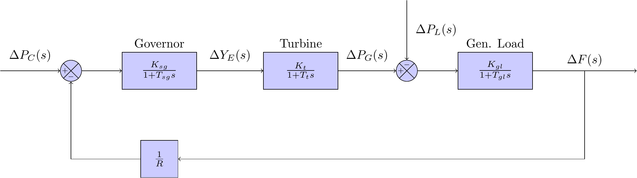
In order to make things simpler to model, researchers often aggregate generators into a group called a power area. Generators are placed into a power area based on characteristics such as geographic location, or the provision of power to a subset of consumers. This simplificaiton is convenient for my purposes because I can use models for a single governor, a single turbine, and a single generator load to model a single area power system. A block diagram of a single area power system can be seen in Figure 1. This particular model is using a proportional feedback loop to control frequency - the literature refers to this as primary control.
MATLAB’s Simulink was used to implement this frequency domain model. The program has a handy dandy GUI for drag and drop building of these types of frequency models - the whole thing took me about 10 minutes to make (and fix up all the bugs). The model parameters were selected based on some of the more common values I had come across in these types of classical models. A full break down of the model parameters, including a description and their assigned values, can be seen in Table 1.
| Description | Parameter | Value |
|---|---|---|
| Speed governor gain | \(K_{sg}\) | 1.00 |
| Speed governor time constant | \(T_{sg}\) | 0.20 |
| Turbine gain | \(K_{t}\) | 1.00 |
| Turbine time constant | \(T_{t}\) | 0.50 |
| Generator load gain | \(K_{gl}\) | 1.25 |
| Generator load time constant | \(T_{gl}\) | 12.5 |
| Speed regulation of the governor | \(R\) | 0.05 |
| Load demand change | \(\Delta P_L\) | 0.02 |
| Speed changer | \(\Delta P_C\) | 0.00 |
The completed Simulink implementation of the block diagram is shown in Figure 2. Note that there are a couple of block elements that are not included in Figure 1. The first is the scope — this is a Simulink element that allows for the recording of simulation signals (it’s a bit like an oscilloscope). The second is the out blocks — these capture data and export it to the MATLAB workspace so you can make pretty plots and stuff.

The simulation was run for exactly 11 seconds. The step change in load demand, , was set to take place at 1 second after the simulation started — this is shown in the topmost plot in Figure 3. The frequency response of the system can be seen in the lowermost plot in Figure 3. Note that the controller can arrest the frequency deviation; however, is unable to restore the frequency to the scheduled value. This is consistent with the analysis that was undertaken in the primary control post.
